 Blog Home
Learning When to Skim and When to Read
The rise of Machine Learning, Deep Learning, and Artificial Intelligence more generally has been undeniable, and it has already had a massive impact on the field of computer science. By now, you might have heard how deep learning has surpassed super-human performance in a number of tasks ranging from image recognition to the game of Go.
The deep learning community is now eyeing natural language processing (NLP) as the next frontier of research and application.
One beauty of deep learning is that advances tend to be very generic. For example, techniques that make deep learning work for one domain can often be transferred to other domains with little to no modification. More specifically, the approach of building massive, computationally expensive, deep learning models for image and speech recognition has spilled into NLP. One can see this in the case of the most recent state-of-the-art translation system, which outperformed all previous results, but required an exorbitant amount of computers. Such demanding systems can capture very complex patterns occasionally found in real world data, but this has led many to apply these massive models to all tasks. This raises the question:
Do all tasks always have the complexity that requires such models?
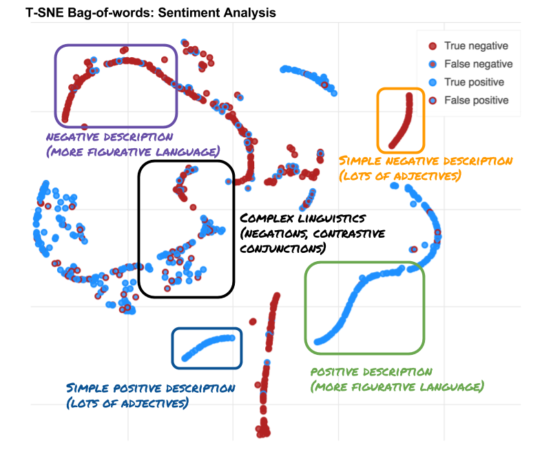
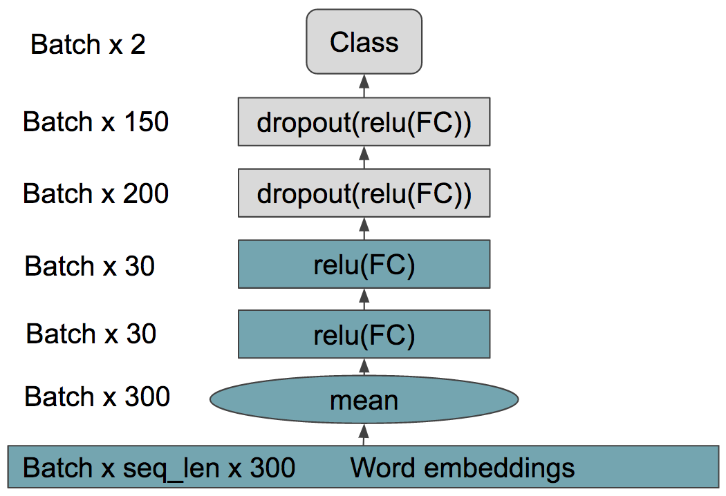
Let's look at the innards of a two layered MLP trained on bag-of-words embeddings for sentiment analysis.

The boundary boxes in the plot above offers some important insights. Real world data comes in different difficulties, some sentences are easily classified while others contain complex semantic structures. In the case of easily classified sentences, running a high-capacity system might be unnecessary. A much simpler model could potentially do an equivalent job. This blog post will explore whether this is the case. It will show that we can often do with simple models.
Deep learning with text
Most deep learning methods require floating point numbers as input and, unless you have been working with text before, you might wonder:
How do I go from a piece of text to deep learning?
A core issue with text is how to represent an arbitrarily large amount of information, given the length of the material. A popular solution has been tokenizing text into either words, sub-words, or even characters. Each word is transformed into a floating point vector using well studied methods such as word2vec or GloVe. This provides for meaningful representations of a word through the implicit relationships between different words.
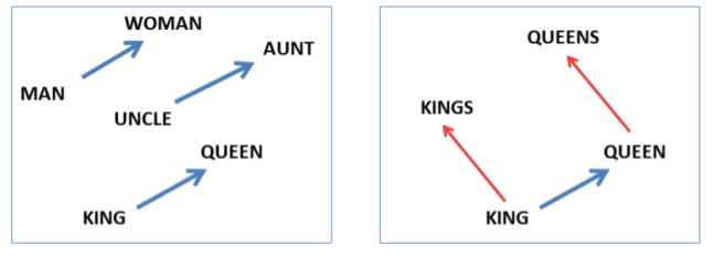
By using tokenization and the word2vec methods we can turn a piece of text into a sequence of floating point representations of each word.
Now, what can we use a sequence of word representations for?
Bag-of-words
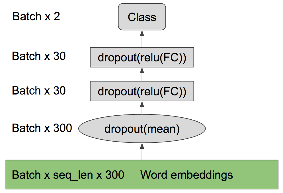
Now let's talk about the bag-of-words (BoW), perhaps one of the simplest machine learning algorithms you will ever learn!
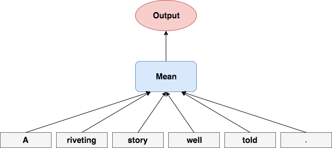
Simply take the mean of the words across each feature dimension. It turns out that simply averaging word embeddings, even though it completely ignores the order of the sentence, works well on many simple practical examples and will often give a strong baseline when combined with deep neural networks (shown later). Furthermore, taking the mean is a cheap operation and reduces the dimensionality of the sentence to a fixed sized vector.
Recurrent neural networks
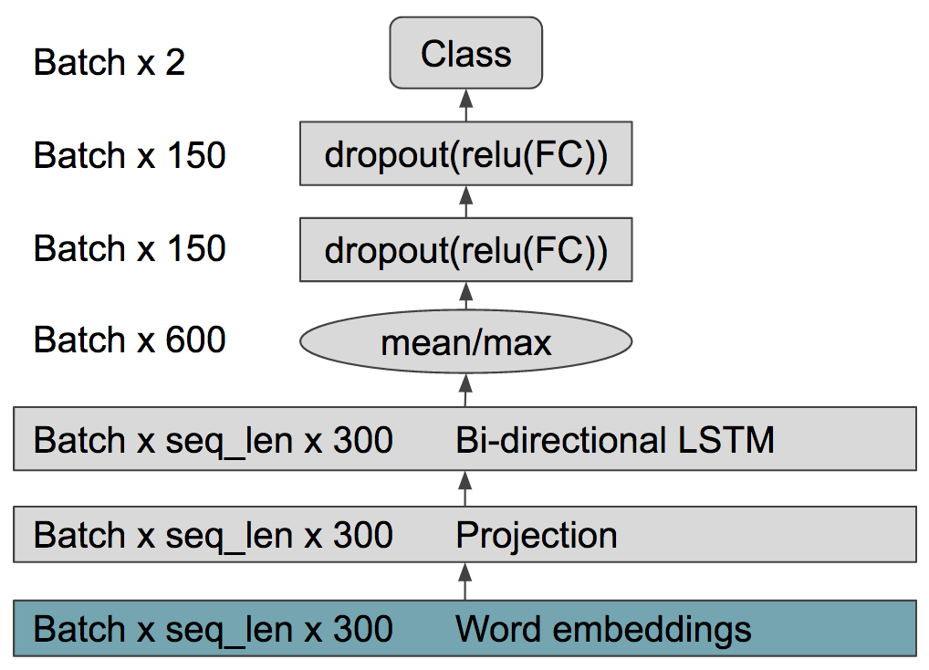
Some sentences require high precision or rely on sentence structure. Using a bag-of-words for these problems might not cut it. Instead, you might want to consider the amazing recurrent neural network!
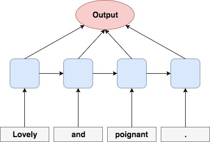
Each word embedding is, in order, fed to a recurrent neural network that then manages to store previously seen information and combine it with new words. When using an RNN powered by the famous memory cells such as the long-short term memory cell (LSTM) or the gated recurrent unit (GRU), the RNN is capable of remembering what has happened in sentences with up to many words! (because of the LSTM's success, the RNN with LSTM memory cells is often referred to as the LSTM). The biggest of these models stack eight of these on top of one another.
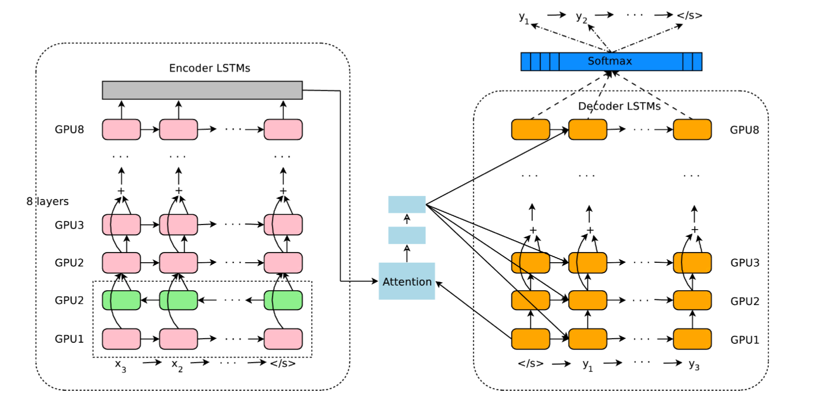
However, the LSTM is much, much more expensive than the cheap bag-of-words model and will often require an experienced deep learning engineer to implement and support efficiently with high-performance computing hardware.
Example: sentiment analysis
Sentiment analysis is a type of document classification for quantifying polarity in subjective passages. Given a sentence, the model evaluates whether it is positive, negative or neutral.
Want to find livid customers on twitter before they start trending? Well, Sentiment Analysis might be just what you’re looking for!
A great public dataset for this purpose (which we will use) is the Stanford sentiment treebank (SST). We have provided a publicly available data loader in pytorch. The SST provides not only the class (positive, negative) for a sentence, but also each of its grammatical subphrases. In our systems we do not utilize any tree information however. The original SST constitutes five classes: very positive, positive, neutral, negative and very negative. We consider the simpler task of binary classification where very positive is combined with positive, very negative is combined with negative and all neutrals are removed.
We have provided a brief and technical description of our model architecture. The important point is not exactly how it is structured, but the fact that the cheap model gets 82% validation accuracy and takes 10 ms for a 64 sized batch, and the expensive LSTM achieves a significantly higher 88% validation accuracy but costs 87 ms for a 64 sized batch (Top models will be in the 88-90% accuracy ballpark).
The cheap skim reader
On some tasks, algorithms can perform at near human level accuracy, but obtaining this performance might burn a hole in the server budget. You also know that if it is not always necessary to have an LSTM powerhouse with real world data, we might be just fine with the cheaper bag-of-words. But what happens when you get a sentence such as this:
"Horrible cast, complete lack of reality, …, but I loved it 9/10”
The order agnostic bag-of-words will surely missclassify with the overwhelming amount of negative words. Completely switching to a crummy bag-of-words would drop our overall performance, which doesn’t sound that compelling. So the question becomes:
Can we learn to separate ‘easy’ and ‘hard’ sentences?
And can we do so with a cheap model to save time?
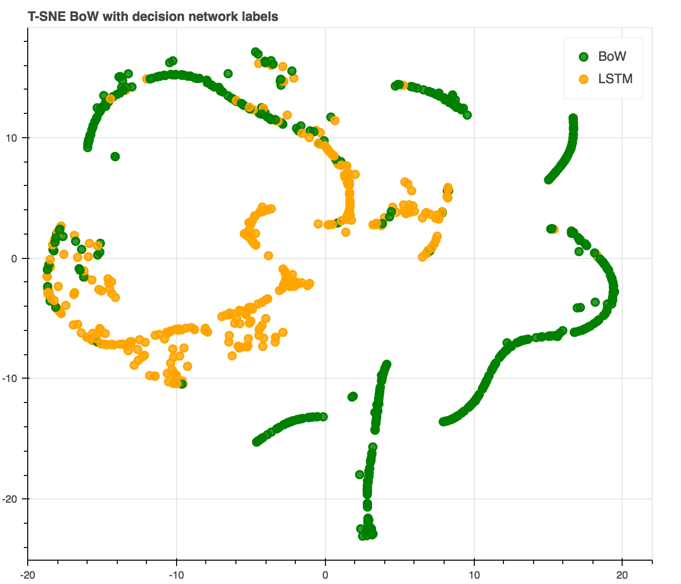
Exploring the innards
A popular way of exploring deep learning models is by plotting how each sentence is represented in the hidden layers. However, as the hidden layers are often high dimensional, we can use algorithms such as the T-SNE to reduce dimensionality to 2D, allowing us to plot it for human inspection.
T-SNE plots are vulnerable to many over-interpretations, but a few trends might strike you.
Interpretations of T-SNE
- The sentences fall into clusters. The clusters consitutes different semantic types.
- Some clusters lie along a simple manifold with high confidence and accuracy.
- Other clusters are more scattered with low accuracy and low confidence.
- Sentences with positive and negative consituents are difficult.
Let's now look at a similar plot for the LSTM.
You can move around, zoom, save and hover over the data points to see their informations. Notice that the tooltip might work better if it is rendered to the right (move the data points to the left side).
Same setup as with the bag-of-words, explore the innards of the LSTM!
We can assess that many of these observations hold true for the LSTM as well. However, the LSTM only has relatively few examples with low confidence, and cooccurrence of positive and negative consituents in sentences does not look to be as challenging for the LSTM as it is for the bag-of-words.
It seems the bag-of-words has been able to cluster sentences and use its probability to identify whether or not it is likely to give a correct prediction for the sentences in that cluster. From these observations, a reasonable hypothesis could be
Confident answers are more correct.
To investigate this hypothesis, we can look at probability thresholds.
Probability thresholding
The bag-of-words and LSTM are trained to give us probabilities for each class, which we can use as a measure of certainty. What do we mean by this? If the bag-of-words returns a 1, it is very confident in its prediction.
Often when predicting we would take the class with the highest likelihood provided by our model. In the case of binary classification (e.g. positive or negative) the likelihood has to be over 0.5 (or else we would be predicting the opposite class!). But a low likelihood for the predicted class might indicate that the model was in doubt. Say the model predicted 0.49 for negative and 0.51 for positive, it might not be so convincing that it actually is positive.
When we say that we threshold, what we mean is that we compare the predicted probability to a value and assess whether or not to use it. E.g. we could decide that we use all sentences with a probability above 0.7. Or we look at the interval 0.5-0.55 to see how accurate predictions with this confidence are, which is exactly what we will investigate in the next plot.
On the threshold plot, the height of the bar corresponds to the accuracy of data points within two thresholds and the line is analogous to the accuracy when using all data points beyond a given threshold.
In the data amount plot, the height of the bar corresponds to the amount of data reciding within two thresholds and the line is the accumulated data from each threshold bin.
From the bag-of-words plots it might occour to you that increasing the probability threshold increases the performance. From the LSTM plot it is not so obvious, which seems common as the LSTM overfits the training set and only provides confident answers.
Use the BoW for easy examples, and the pristine LSTM for difficult ones.
Thus, simply using the output probability could give us an indication of when a sentence is easy and when it is in need of guidance from a stronger system, like the powerful LSTM.
Using the probability threshold, we create a strategy which we refer to as the "probability strategy", such that we threshold the probability of the bag-of-word system, and use the LSTM on all data points not reaching the threshold. Doing so provides us with an amount of data used for the bag-of-words (sentences above the threshold) and a set of data points where we have either chosen the BoW (above the threshold) or the LSTM (below the threshold), which we can use to find an accuracy and cost of computing. We then get a ratio between the BoW and the LSTM increasing from 0.0 (only using LSTM) to 1.0 (only using BoW), which we can use to calculate the accuracy and time to compute.
Baseline
To construct a baseline we consider the ratio between the two models, e.g. 0.1 data used for BoW would correspond to 0.9 times LSTM accuracy and 0.1 times BoW accuracy. The purpose is to have a baseline with no guided strategy where the choice of using BoW or LSTM on a sentence is randomly assigned. However, there is a cost to using the strategies. We have to run all of the sentences through the bag-of-words model first, to determine if we should use the bag-of-words or the LSTM. In case that none of the sentences reaches the probability threshold, we could be running an extra model for no good reason. To incorporate this, we calculate the cost of our strategies and the ratio in the following way.
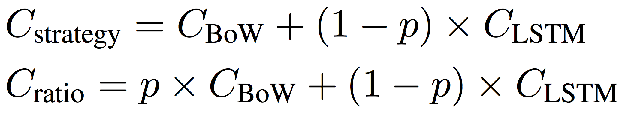
Where C is the cost and p the proportion of data used for bag-of-wordsResults on the validation set comparing the accuracy and speed from different ratio combinations between BoW and LSTM (red line) and the probability thresholding strategy (blue line) Data points to the far left corresponds to only using a LSTM while the far right corresponds to only using the bag-of-words, in between corresponds to mixes of the two. The blue line represents using a combination of CBOW and LSTM with no guided strategies, while the red curve depicts using the bag-of-word probability as a strategy to guide which passages to use which system for. Hover over the lines to see time saved for each ratio/probability threshold. Notice that maximum time saves is ~90% as this corresponds to only using bag-of-words.
The interesting discovery is that we find that using the bag-of-words thresholds significantly outperforms not having a guided strategy.
We then measure the average value on the curve, which, we refer to as Speed Under the Curve (SUC). As shown in table below.
| Strategy | Validation SUC |
|---|---|
| Ratio between BoW and LSTM | 84.84 |
| Probability | 86.03 (std=0.3) |
Learning when to skim and when to read
Knowing when to switch between two different models is not enough. We want to build a more general system that learns when to switch between each model. Such a system would help us deal with the more complicated behaviour of
Can we learn when reading is strictly better than skimming in a supervised way?
Where "reading" is using the LSTM which goes from left to right and stores a memory at each time step and "skimming" is using the BoW model. When operating on the probability from the bag-of-words model we make our decision based on the invariant that the more powerful LSTM will do a better job when the bag-of-word system is in doubt, but is that always the case?
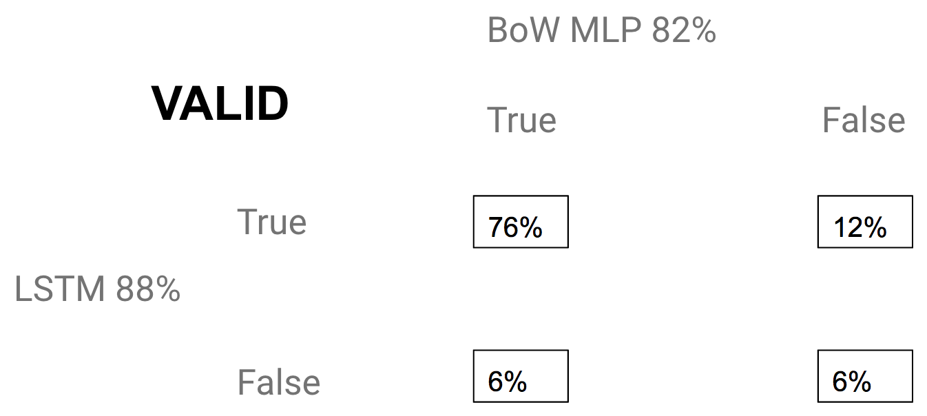
In fact, it turns out that it is only the case 12% of the time, whereas 6% of the sentences neither the bag-of-words or the LSTM get correct. In such case, we have no reason to run the LSTM and we might as well just save time by only using the bag-of-words.
Learning to skim, the setup
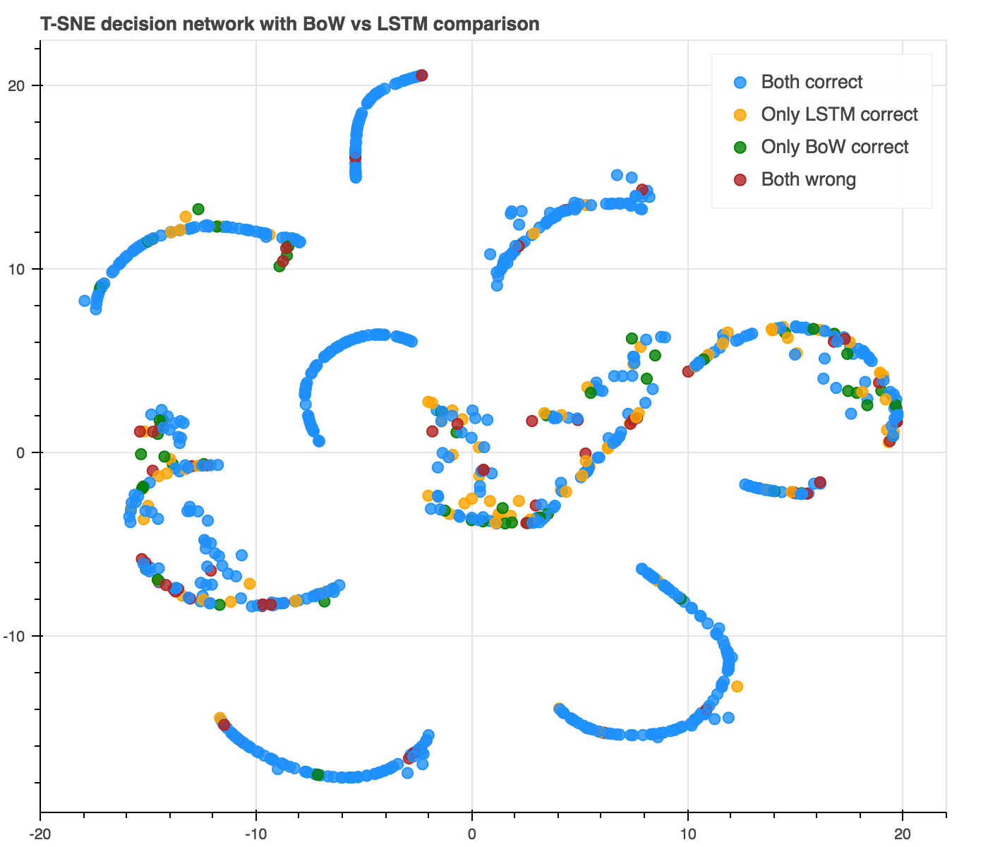
So we don’t always want to use the LSTM when the BoW is in doubt. Can we make our bag-of-word model understand when the LSTM also might be wrong and when we should spare our precious computational resources? Let us look at the T-SNE plot again, but now with the confusion matrix between the BoW and the LSTM plotted. We hope to find a relationship between the elements of the confusion matrix, especially when the BoW is incorrect.
From the comparison plot, we find that it is easy to assert when the BoW is correct and when it is in doubt. However, there is no clear relationship between when the LSTM might be right or wrong.
Can we learn this relationship?
Further, the probability strategy is quite restrictive as it relies on an inheritent binary decision and requires probabilities. Instead, we propose a trainable decision network that is based on a neural network. If we look at the confusion matrix, we can use that information to generate labels for a supervised decision network. In this way, we would only use the LSTM in the cases where the LSTM is correct and the BoW is wrong.
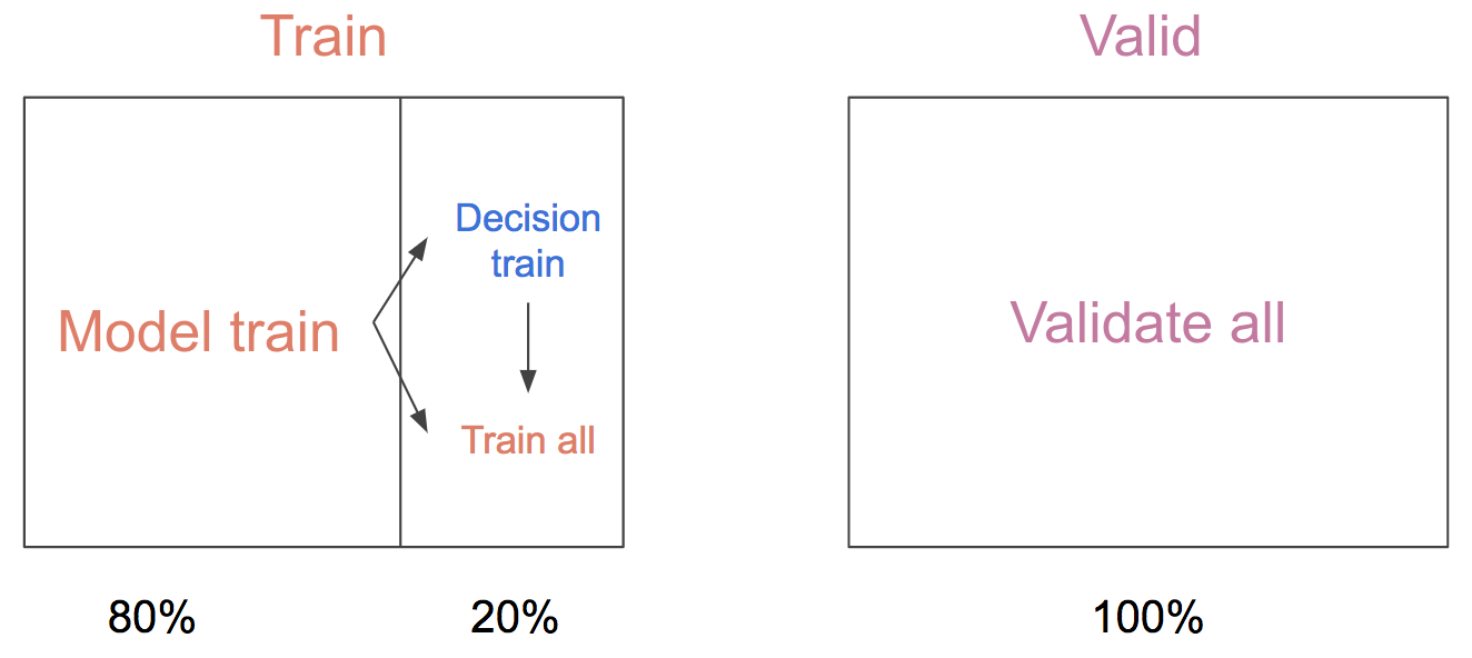
To generate the dataset, we need a set of sentences having the true, underlying, prediction of our bag-of-words and the LSTM. However, during training the LSTM will often achieve upwards 99% training accuracy, significantly overfitting the training set. To avoid this, we split our training set into a model training set (80% of training data) and a decision training set (remaining 20% of training data) that the model has not yet seen. Afterwards we fine-tune our model with the remaining 20%, hoping that the decision network will still generalize to this new, unseen, but very related and slightly better system.
To build our decision network, we tap into the last hidden layer of our cheap bag-of-words system (the same layer we used to generate our T-SNE plots). We then stack a two layer MLP on top of our bag-of-words training on the model training set. We found that if we do not follow this recipe, the decision network will not be able to learn the tendencies of the BoW model and will not generalize well.
The classes chosen on the validation set by the decision network, based on the models trained on the model training set, is then applied to the full, but very related, models on the full training set. The reason why we apply it on the model trained on the full training set, is that the models on the model training set will often be inferior and thus result in a lower accuracy. The decision network is trained with early stopping, based on maximizing the SUC on the validation set.
How does our decision network perform?
Let us start by looking at the predictions of the decision network.
Notice how closely this resembles the probability cutoff of the bag-of-words. Now let us look at the T-SNE of the last hidden layer of the decision network, to see if it is actually able to cluster some information of when the LSTM is correct or wrong.
It seems the decision network is capable of picking up the clustering from the hidden states of the bag-of-words. However, it does not seem like it is able to understand when the LSTM might also be wrong (clustering yellows from reds).
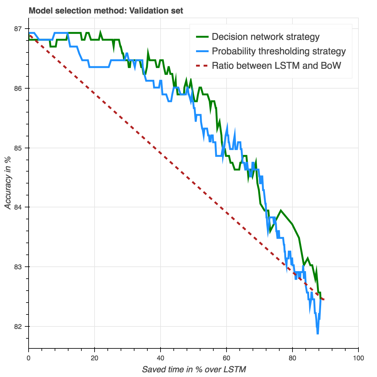
From the data accuracy over saved time curves, it is not obvious whether or not the decision network is better.
| Policy | Validation SUC | Test SUC |
|---|---|---|
| Ratio between BoW and LSTM | 84.84 | 83.77 |
| Probability | 86.03 (std=0.3) | 85.49 (std=0.3) |
| Decision network | 86.13 (std=0.3) | 85.49 (std=0.3) |
From prediction plot, data amount vs. accuracy and SUC score we can infer that the decision network is splendid at understanding when the BoW might be correct and when it is not. Further, it allows us to build a more general system that taps into the hidden states of deep learning models. However, it also goes to show that it was very difficult to make the decision network understand the behaviour of systems that it did not have access to, such as the more complex LSTM.
Discussion
We now know that large powerful LSTMs can achieve near human-level performance on text, that not all real-world data needs near human-level performance, that we can train a bag-of-words model to understand when a sentence is easy and that using bag-of-words for easy sentences allows us to save a significant amount of computation time with only a minor drop in performance (depending on how aggressive we threshold the bag-of-words).
This approach is related to mean averaging usually performed when model ensembling as often the model with high confidence will be used. However, by having an adjustable confidence from the bag-of-words and not needing to run the LSTM, we can decide how much computation time vs. accuracy savings we are interested in. We believe that this method will be useful for deep learning engineers looking to save computational resources without having to sacrifice performance.
Citation credit
Alexander Rosenberg Johansen, and Richard Socher. 2017.
Learning when to skim and when to read
By having a better understanding of when a deep learning system might be wrong, we can make informed decisions about when to use which deep learning model. This allows us to save computational time by only running the bare minimum to complete a task.