Blog Home
Interpretable Counting for Visual Question Answering
Learning to answer open-ended questions about images, a task known as visual question answering (VQA), has received much attention over the last several years. VQA has been put forth as a benchmark for complete scene understanding and flexible reasoning, two fundamental goals of AI. But, apart from accurate answers, what would these milestones look like in a successful VQA model? When it comes to the visual component, one line of thinking points to scene-graphs. In a scene-graph, an image is organized into the underlying objects, their attributes, and the relationships between object pairs. This kind of organization is very easy to understand because each element of the scene (‘person’, ‘dog’, ‘next to’, etc.) gets its own representation. Capturing the image this way could provide a fairly ideal scaffold for extracting information relevant to answering a given question.
Thinking about VQA this way brings another consideration into focus: interpretability. If the representation of the image is easy to interperet, can we use that property to make an AI that's easier to understand? A central idea here is that interpretability requires a reasoning process that is grounded in discrete visual representations and that preserves that discrete organization when forming an answer. Here, we zoom in on this notion of discrete representation and explore a subtask within VQA that has been met with particular difficulty: counting. Counting questions offer an ideal entry point for exploring networks built with the goal of interpretability in mind, such as the one we introduce here, which we call Interpretable Reinforcement Learning Counter (IRLC).
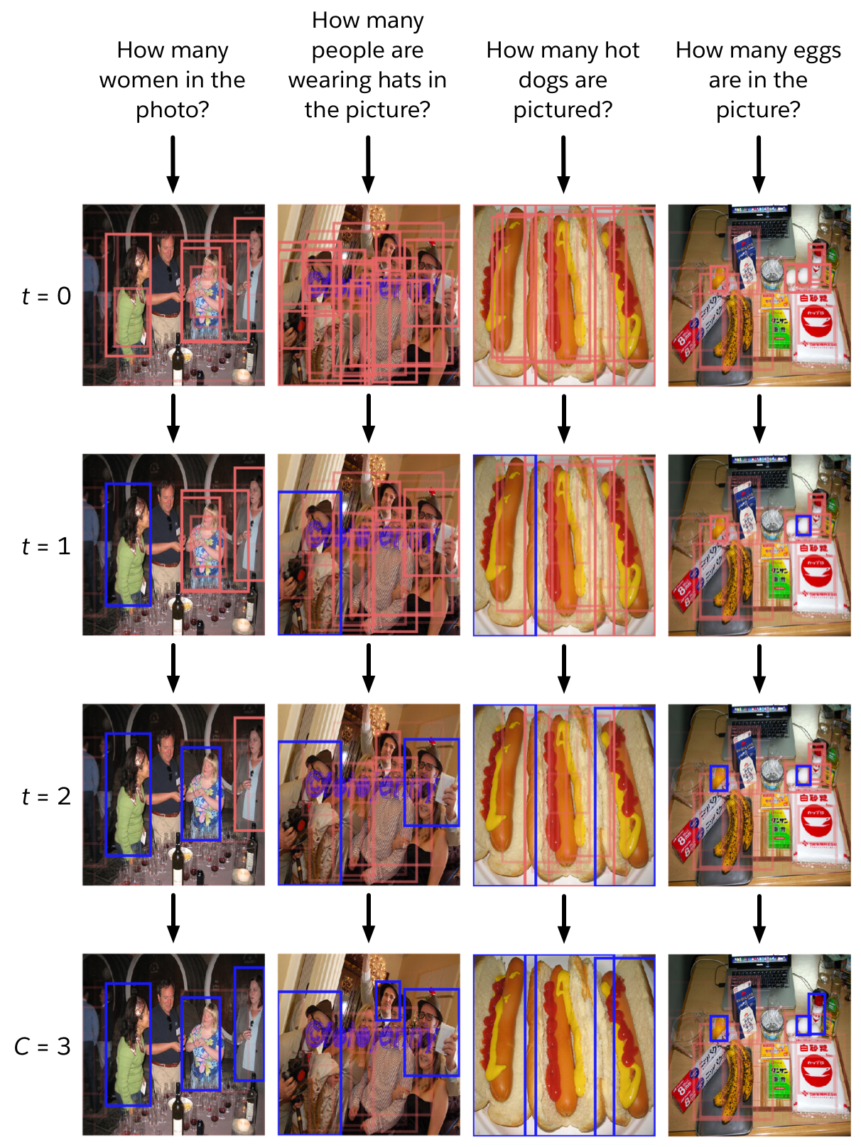
Our model learns to count by enumerating relevant objects in the scene, formulated as the process of sequentially deciding which object to add to the count. We model how the choice to count one object affects the way other objects are used in subsequent steps and train the network using reinforcement learning (RL). For all our experiments, we represent the image as the set of object proposals generated from a pre-trained vision module. Figure 1 shows an example of IRLC in action. The inputs are the question and the object proposals from the vision module. IRLC uses the question to give each object an initial score, then cycles through picking the highest-scoring object and updating the scores based on the selection. When none of the remaining objects have a high enough score, the process terminates, giving a count equal to the number of selected objects.

After training on counting questions, IRLC outperforms the other baselines we experimented with, including a model adapted from the current state of the art for VQA. In addition, IRLC points to the exact object proposals on which each count is based. In other words, it returns visually-grounded counts. Compared to the attentional focuses produced by a more conventional model, we argue that the visually-grounded counts of IRLC provide a simpler and more intuitive lens for interpreting model behavior.
Models and approach
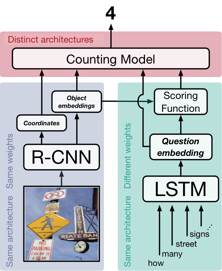
Figure 2 shows the general pipeline we experiment with. There are 3 basic stages. In the first stage the image is processed (blue-shaded area), returning a set of object proposals and the estimated relationships between objects. Each object comes with a bounding box, telling us where in the image it is, and a vector encoding, which captures the features of the object. Anderson et al. (2017) trained an object detector as part of their work which led to state of the art in VQA; the detection outputs of their model are publicly available, so we use them here. In the second stage (green-shaded area), we use an LSTM RNN to get a vector encoding of the question. We estimate the relevance of each object proposal to the question by comparing the question and object embeddings using a scoring function, which is set up as a single feedforward layer in the network. In the third stage (red-shaded area), we use the outputs of the previous 2 stages to generate a count. We experiment with three strategies, each of which is defined by a distinct counting module.
We set up our work this way for a few reasons. In particular, previous studies don’t train on or report performance on counting specifically, so we need to do those experiments ourselves. In addition, setting the experiments up this way lets us control for many of the little decisions that likely affect absolute performance. For example, by using object proposals from the pre-trained model to serve as the vision module, we ensure that all our counting models use the same visual features. We want to isolate the effects due specifically to the design of the counting module.

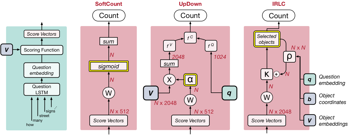
The simplest of the three models we test generates a count by converting each object proposal into a fractional value (by applying a sigmoid function to the score value) and then taking the sum over all of them. Because each of these values is somewhere between 0 and 1, we call this approach SoftCount (Figure 3, middle-left).
We also implement a more typical style of VQA architecture, which we design after Anderson et al. (2017)--see also Teney et al. (2017). The key to this approach is that the score values are used to compute attention weights for each object proposal. This gives each proposal a weight between 0 to 1, such that all the weights sum up to 1. Rather than take the sum of these values (as in SoftCount), we use the attention weights to compute a weighted average of the object encodings, as if combining all the object encodings into a single, representative object. We use the weighted average of the object encodings and the question encoding to estimate the count (which requires us to treat the count as a class in a classification problem). We refer to this architecture as UpDown (Figure 3, middle-right).
Lastly, we introduce Interpretable Reinforcement Learning Counter--or IRLC for short. With IRLC, we aim to learn how to count by learning what to count. We assume that each counting question implicitly refers to a group of objects within the scene that meet some criteria. In this sense, the goal of IRLC is to enumerate each of the objects in that group. This means that, when generating a count, IRLC must choose which specific object proposals it wants to include in the count. We model this process as a sequence of discrete choices.
Figure 3 (far-right) gives a schematic for the counting module of IRLC. Like the other two counting strategies, this one begins with the scores assigned to each object proposal and converts them into a set of selection probabilities, illustrated as κ. We select the object proposal with the largest κ value and add it to the counted objects. Importantly, we also model how each choice affects subsequent decisions. This is controlled by an interaction matrix, illustrated as ρ (which is the output of a feedforward neural network that takes the question, the object encodings, and their coordinates). This sets up a sequential decision process where each step has 2 phases. In the first step, we pick which object to add to the count--call this object i. Then, we take the ith row of the interaction matrix, ρ, and use it to update the selection probabilities--that is, we add the ith row of ρ to κ. Each object can only be selected once. We repeat this process until all remaining κ values are below a learnable threshold, at which point the decision is made to stop counting and the returned count is equal to the number of selected objects.
Importantly, our training data doesn’t label the objects that are relevant to the question, it only gives us the final answer. So, all we can tell our model during training is how far away the estimated count was from the ground truth. Because of this restriction and the discrete nature of the counting choices, we train using RL. Since κ can be interpreted as a set of selection probabilities, our approach is well suited for policy gradient methods. We specifically use Self-Critical Sequence Learning, which involves stochastically sampling object selection decisions using the probabilities given by κ and comparing the outcome to what happens if objects are chosen greedily (as at test-time and described above). The network is trained to increase (decrease) the probability of selection sequences that did better (worse) than the greedy selection.
Counting in VQA
Typically, studies on VQA provide performance metrics for each of 3 question categories: ‘yes/no’, ‘number’, and ‘other’. For our purposes, we need to be more precise, because the ‘number’ category includes both counting and non-counting types of questions. To deal with this, we construct a new combination of the training data from the VQA v2 and Visual Genome datasets. We isolate the questions that require counting and whose ground truth answer is in the range of 0-20. For development and testing, we apply the same filter to the validation data from VQA v2. We set aside 5000 of those questions as our test split and use the rest for development (i.e. early stopping, analysis, etc.). We call this dataset HowMany-QA.
Performance
We trained each of the model variants described above on the training split of HowMany-QA. We rely on 2 statistics to evaluate the counts produced by the models. The first of these metrics is accuracy--which is the standard metric for VQA. This simply tells us how often the best guess of the model was correct, so higher is better. However, accuracy doesn’t capture the typical scale of the error, so we also want to capture how far, on average, each model’s answers were from the ground truth. For that, we also calculate the average squared error of the estimated counts and take the square root of that value (root mean squared error, or RMSE). Since RMSE measures error, lower is better. These values are shown the following table:
| Model | Accuracy | RMSE |
|---|---|---|
| SoftCount | 50.2 | 2.37 |
| UpDown | 51.5 | 2.69 |
| IRLC | 56.9 | 2.39 |
A couple things stand out. First, IRLC is substantially more accurate than the other two baselines (SoftCount and UpDown). Second, the two baselines trade-off accuracy and RMSE. That is, SoftCount returns counts that are on average closer to the ground truth than UpDown (lower RMSE) but are less often exactly correct (lower accuracy). So, these two metrics capture subtle differences in the quality of the counting performance. This underscores the observation that IRLC performs strongly in both metrics.
Qualitative results
The quantitative performance of IRLC shows that a discrete decision process built on discrete visual representations is not only viable for counting in VQA but superior to alternative methods. But what about our intuition that such an approach should also simplify interpretation of model behavior? There’s no clear metric for saying whether one model is more interpretable than another, but Chandrasekaran et al. (2017) have made some progress in bringing this idea into the experimental realm. For now, we’ll form a more qualitative argument by borrowing a central idea from their work: that a key hallmark of interpretability is the ability to understand failure modes.

Rather than provide an exhaustive set of examples for some failure mode, we illustrate a pair of failure cases that exemplify two trends observed in IRLC; these are shown in Figure 4. These two cases also led to failures in the UpDown model, so we include its outputs and attention focuses for comparison. IRLC has little trouble counting people (the most frequently encountered counting subject in the training data), but, as shown in the left example, it encounters difficulty with referring phrases (in this case, “sitting on the bench”) and fails to ignore 2 people in the foreground. In the right example, the question refers to “ties,” a subject for which the training data has only a handful of examples. When asked to count ties, IRLC includes an irrelevant object--the man's sleeve. This reflects the broader tendency for IRLC to have difficulty identifying the relevant object proposals when the question refers to a subject that was underrepresented during training. The nature of these failures are obvious by virtue of the grounded counts, which point out exactly which objects IRLC counted. In comparison, the attention focus of UpDown (representing the closest analogy to a grounded output) does not identify any pattern. From the attention weights, it is unclear which scene elements form the basis of the count returned by UpDown.
We invite the reader to evaluate for him/herself whether IRLC succeeds in providing more interpretable output than the alternative approaches. Below, we provide a broader set of examples and the outputs from each model (Figure 5). In addition, we illustrate how the sequential decision process evolves while IRLC counts for each of several examples (Figure 6).
Conclusion
We present an interpretable approach to counting in visual question answering, based on learning to enumerate objects in a scene. By using RL, we are able to train our model to make binary decisions about whether a detected object contributes to the final count. We experiment with two additional baselines and control for variations due to visual representations and for the mechanism of visual-linguistic comparison. Our approach surpasses both baselines in each of our evaluation metrics. In addition, our model identifies the objects that contribute to each count. These groundings provide traction for identifying the aspects of the task that the model has failed to learn and thereby improve not only performance but also interpretability.
Citation credit
Alexander Trott, Caiming Xiong, and Richard Socher. 2017.
Interpretable Counting for Visual Question Answering