Improving Graph Convolutional Networks with Lessons from Transformers

15 min read

Michael Sollami

Improving Graph Convolutional Networks with Lessons from Transformers

Post written by Cameron Wolfe

Introduction

Graph Convolutional Networks (GCNs) and Graph Attention Networks (GATs) can understand and classify patterns in structured graph data. Many different relationships can be encoded in a graph’s topology, which makes these models extremely expressive. Additionally, the formulation of GCNs enables them to generalize to arbitrary graphs after training. They can classify unseen graphs or generalize to new structures in a test set. GCNs may be utilized for a wide spectrum of tasks such as semi-supervised classification over citation graphs, e-commerce product classification, and even language modeling. In fact, transformers can be fully expressed as a GCN, demonstrating the generality of this architecture [1]. Furthermore, due to new advances in tooling for deep learning, GCNs may be easily implemented, accelerated with the use of a GPU, and even batched to process multiple graphs in parallel [2].

GCNs are currently the state-of-the-art for deep learning on graphs, but you may wonder in what practical scenarios are these methods most applicable. Well, many common neural components, such as self-attention, can be re-expressed with a graphical structure, which enables tasks such as language translation to be performed with a GCN. Many industrial deep learning systems build knowledge graphs to concisely represent relationships containing within vast amounts of data [3]. Additionally, streaming and e-commerce platforms easily represent users and their relationships using a graph structure, giving rise to new opportunities in effective recommendation systems. Overall, these neural networks serve as a state-of-the-art tool for performing deep learning on graph-structured data, making them a useful addition to any data scientists tool belt as graph-like data becomes more prevalent.

Transformer architectures have revolutionized deep learning for textual data [4, 5, 6], data with multiple modalities [7, 8, 9, 10], and much more (even object detection! [11]). Given the recent success of the transformer architecture and the many similarities between transformers and GCNs, we found it quite surprising that the GCN architecture has not gained as much popularity. The attention representation within a GCN can express self-attention employed within transformer layers, and can even generalize to sparse attention representations across the graph, thus making them an interesting tool for future research in various domains. Interestingly, the implementation details of GCNs, as well as provided implementations online, seem to lack some common components of the transformer architecture, such as concatenation and projection of head output and intermediate layer normalization. This blog post aims to unify some of these architectural differences and improve overall performance of the GCN by taking some lessons from transformers.

The purpose of the article is twofold. First, we introduce the basic background regarding GCNs and GATs, as well as explain how the originally-proposed architecture of these models can be implemented. Second, we draw parallels between the Transformer and GCN architectures by highlighting aspects of the Transformer architecture that are missing from the vanilla GCN. By adding these architectural components into the GCN models, performance can be improved and training accelerated. Most importantly, we hope to provide a comprehensive outline of the information needed to implement a deploy a GCN, enabling practitioners to quickly adopt these architectures for related applications.

Background

Deep Learning for Graphs

Because deep learning on graph data is relatively novel, we find it necessary to specify the formulation of deep learning for graphical data. The input data for a graph convolutional network consists of a single graph or a batch of graphs. Within each graph, each node has an associated embedding. Furthermore, there are various connections between the nodes of each graph, and these connections may be arbitrary. Given these graphs and their associated input embeddings, deep learning on graphs typically performs some kind of classification, either for each node within a graph or for the graph as a whole.

Two major problem types exist for classifying graphs: transductive and inductive tasks. In transductive tasks, the structure of the graphs used for classification is known a priori. Therefore, the model does not need to generalize to unseen structures and graphs that may be encountered in a test set. Rather, the model is simply expected to learn patterns of classification for nodes of a graph with known structure (e.g., semi-supervised classification, where only a portion of the nodes have labels). In contrast, inductive tasks do not assume knowledge of graph structure. As a result, these tasks must generalize to entirely new graphs that have not been seen during training.

Graph Convolutional Networks

GCNs are neural networks designed to perform convolutions over undirected graph data [12]. Originally proposed as a method for performing semi-supervised classification over the nodes of graphs, their applications were later extended to other tasks. A single layer within a GCN can be described by the following equation:

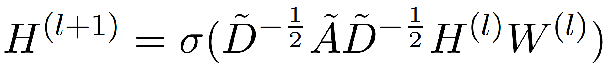
Here H represents the node embeddings within a graph, W represents a projection matrix, A represents the adjacency matrix of the graph with added self-connections, D represents a diagonal matrix that stores the degree of each node, and sigma represents an element-wise nonlinearity. The equation simply projects the node embeddings, computes each new embedding as the average of all of a node’s neighbors, and applies an element-wise nonlinearity to the new embeddings. These operations comprise a single graph convolutional layer, and these layers can be stacked to build a GCN.

Notice that this formulation requires the entire adjacency matrix of the graph within its forward pass. Thus, the complete structure of a graph must be known before performing classification. The GCN is restricted to transductive tasks, creating the need for a more generalizable formulation of graph convolutions.

Graph Attention Networks

GATs are very similar to GCNs, but can be applied to both transductive and inductive tasks [12]. We apply the same convolutional layer as seen in the GCN, but use attention over each node’s neighboring embeddings instead of taking an average. This formulation enables the model to assign different importances to nodes within the same neighborhood, increasing its capacity. Furthermore, by formulating the GAT as an attention mechanism over each node’s neighborhood, the model can be applied to arbitrary graph structures without knowing the structure beforehand (i.e., no matter the size of the neighborhood, the operation is the same). The GAT, therefore, can be applied to inductive tasks.

GATs utilize additive attention over a neighborhood [14]. The attention weight for each neighboring node is calculated by passing the neighbors embedding, concatenated with the main node’s, through a feed forward neural network, outputing a scalar score. Score normalization is accomplished by using a softmax across all neighboring nodes (i.e., this feed forward network is trained along with the rest of the network). After computing the attention scores of all neighboring nodes, the new embedding for a node is defined as follows:

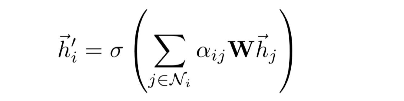
Where W is a projection matrix, alpha represents the attention weights, h is the node embedding, and sigma is an element-wise nonlinearity. These components comprise a single layer of a GAT and many of these layers may be stacked on top of each other. Additionally, similar to transformers, this layer can be generalized to have many heads, the output of which are averaged to create a fixed-sized output embedding after the forward pass.

In the remainder of this post, we focus solely on GATs. We prefer GATs due to their ability to handle inductive classification tasks. Furthermore, GATs can recover the GCN algorithm by setting uniform attention weights for all nodes, performing an averaging operation in each neighborhood. As a result, we lose no representational power by abandoning the GCN for the GAT. Finally, almost all lessons learned from the GAT are readily applicable to the GCN architecture.

Transformers

Because transformers and their similarities to GCNs, are pivotal to the key concepts in this post, we wish to provide a brief summary. We encourage the interested reader to see many other in-depth descriptions that have been provided for transformers [4, 15, 16].

Transformers are comprised of two key operations: self-attention and feed-forward neural networks. Given a set of input token embeddings, one must compute a query matrix, key matrix and value matrix, where each of these matrices are produced by a separate linear projection. This operation can be described as follows:

Where each W represents a separate linear projection, Q is the query matrix, K is the key matrix, V is the value matrix, and X is the input token embeddings. Given these query, key, and value matrices, attention scores can be calculated as follows:

Where d represents the embedding cardinality. Given these attention scores, the matrix product can be taken with the value matrix to yield the output tokens of the self-attention layer. These output tokens are then passed through a feed forward neural network to yield the layer output. Typically, sublayers within the transformer layer are residual and followed by a layer normalization operation. Additional, self-attention is computed across multiple heads, where the output of each head is concatenated and projected to the correct size. These sublayers summarize the basic details of the transformer architecture that will be necessary to understand this post.

Methodology

Vanilla GAT

The GAT architecture, as proposed in [13], works relatively well for both inductive and transductive tasks. This architecture followed all of the specifications provided in the description of a GAT layer, and added a few more tricks for better performance. The model utilized eight attention heads, each with a hidden layer size of eight, yielding an embedding size of 64 when the output of each head is concatenated together. The model has a single hidden layer that is followed by an exponential linear unit (ELU) activation. After the ELU activation a GAT layer with a single attention head is applied to the 64-dimensional output to yield the classification logits (i.e., there is no extra classification layer). During training, the authors apply L2-regularization and two forms of dropout: over the inputted node features to each layer and to the attention weights for each node. Dropout is applied generously, with a probability of 0.6 for most datasets. Furthermore, the authors propose that the architecture may be augmented with residual connections in the hidden layer of the GAT to improve performance.

Improving the GAT

Despite the GATs effectiveness, we found the architecture specifications described above to be somewhat lacking. Though the authors proposed the addition of residual connections, it seemed that the architecture above would have difficulties in training, especially if more and bigger hidden layers were used (i.e., this was also observed empirically). Therefore, I read over the architectural details of the transformers and realized many of the tricks that are used for building effective transformers can also be applied to GATs. These architectural “tricks” that we added to the GAT are as follows:

LayerNorm: Transformers typically follow each sublayer (i.e., self-attention of FFNN) with both a residual connection and a layer normalization operation. We added this to the GAT architecture by performing layer normalization both following the projection of the node embeddings and after the new node embeddings have been created (i.e., after the values are aggregated with attention across all neighbors). Additionally, residual connections were added in all hidden layers, as originally suggested in [13]. These modifications were made in an attempt to stabilize training and enable the use of deeper architectures.
Attention Normalization: In [4], authors propose that dot product attention, prior to applying softmax, should be normalized by the square root of the cardinality of the embeddings being used. By doing this, one can ensure that the dot product, as the embedding size grew, would not yield large values that create very small gradients in softmax. Although GATs employ additive attention, a similar concept can be used to yield better training by normalizing the input to attention by the square root of the dimensionality of the embeddings. In doing this, one ensures that the resulting attention scores have smaller magnitude, making it less likely for vanishing gradients to appear in the softmax computation.
Projection of Head Output: GATs concatenate the output of all heads to yield the embeddings that are passed into the next layer for each node. Therefore, if eight heads are used, each with an embedding size of eight, the node embeddings would begin with a size of 64 in the next layer. In contrast, the transformer architecture handles the output of multiple heads by concatenating the output, and projecting this larger, concatenated embedding to be the size of the original size. Applying this idea to GATs, one can drastically increase the embedding sizes that are used without significant computation overheads. For example, the hidden size of the GAT can be set to 64 for all eight heads. The output of these heads, once concatenated together, can then be projected by a learnable weight matrix to a size of 64, yielding embeddings of the same size that are passed to the next layer. Projecting head outputs to maintain embedding size allowed the hidden size of the network to be significantly increased with minimal overheads, resulting in significantly improved performance.
Adding a Classification Layer: The final peculiarity in the GAT architecture was the fashion in which classification was performed. Namely, a GAT layer was applied that yields an output with the same size as the logits. Although there is nothing wrong with performing classification in this way, I though it would be more natural to add an extra, linear classification layer on top of the embeddings produced by the stacked GAT layers. We maintained the same size of embeddings throughout all layers. Once the final node embeddings were produced (i.e., following the final multi-headed GAT layer), we created an extra linear layer that projects each of the node embeddings to the correct size for classification, creating a specific layer that is used for classification. This modification allows the multi-headed GAT layers to focus on creating useful node embeddings that can then be used for classification by a separate layer, separating the representation and classification aspects of the network into distinct components.

Through adding each of these proposed changes to the originally proposed GAT architecture, we significantly accelerated the model’s training, as well as improve its performance over some larger datasets.

Implementation Details

The GAT that we utilized for these experiments was created using the deep graph library (DGL) [17] and PyTorch. We found that DGL provides a very intuitive, easy-to-learn interface for working with graph data in Python, which easily integrates with PyTorch. The final network that we used had two hidden layers, each with eight heads and embedding sizes of 64. The head output was projected using a learnable linear layer to maintain a hidden size of 64 throughout the network. We applied both attention score and node embedding dropout generously throughout each task. All hidden layers were augmented with Residual connections. Layer normalization was applied at all layers as described above. All models were trained with the same weight decay as originally proposed in [13]: 5e-4.

Experiments

We tested the proposed architectural changes to the GAT across both inductive and transductive tasks. Overall, we tried to use datasets for my experiments that are readily available through DGL [18], so that all of these experiments can be easily replicated. The datasets that I used to evaluate the proposed architecture are as follows:

Cora (Transductive): The Cora dataset [19] is a graph of scientific publications, where each node represents a publication and the connections represent citations of one publication to another. Each node, or publication, can be classified as one of seven classes. The input of each node is represented by a one-hot bag-of-words (BOW) that is created from the associated publication. We utilize the official training/testing split for the Cora dataset in all of my experiments.
Amazon Co-Purchase Dataset (Transductive): The Amazon Co-Purchase dataset [20] contains a portion of co-purchase e-commerce product datasets obtained via Amazon.com. The nodes represent products on the e-commerce website, while edges indicate that two products are frequently purchased together on the e-commerce platform. Again, node feature inputs are BOW vectors obtained using product review on the e-commerce site. The goal is to predict the semantic class of each node or product within the graph. We utilize a random 20-80 train-test split to evaluate results in all of my experiments.
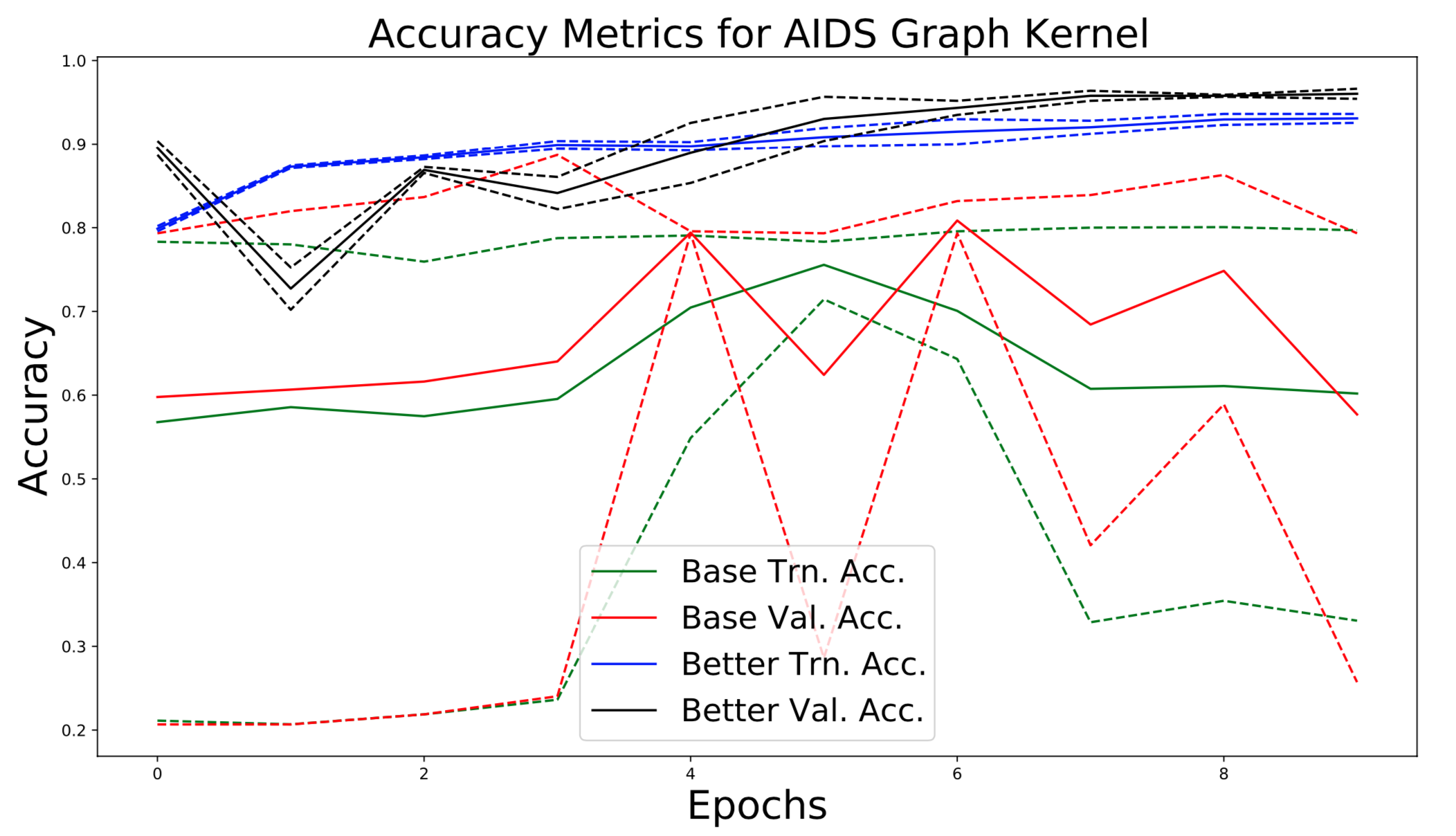
AIDS Graph Kernel Dataset (Inductive): The AIDS graph kernel dataset was taken from [21]. It is a binary classification problem over graph-structured data representing AIDS occurrence. The entire dataset is composed of 2000 unique graphs in total. Each graph has an average of 15.69 nodes and 16.2 edges and is associated with a single binary label. Each node has a single 4-dimensional embeddings associated with it that is used as input to the GAT model. For the experiments performed below, a 80-20 split was performed between training and testing sets.
Protein-Protein Interaction Dataset (Inductive): A small dataset of protein-protein interactions that can be used for inductive graph classification. The training set contains 20 unique graphs (i.e., it is a small subset of a larger dataset), while the testing set contains 2 graphs. Each graph has an average of 2372 nodes. Furthermore, each node has an input feature embedding of size 50, as well as 151 tags/labels that are associated with it. This is a simplified, small protein-protein interaction (PPI) dataset, but it is made available publicly through DGL.

Implementation Details

The GAT that we utilized for these experiments was created using the deep graph library (DGL) [17] and PyTorch. I found that DGL provides a very intuitive, easy-to-learn interface for working with graph data in Python, which easily integrates with PyTorch. All models were trained with the original weight decay proposed in [13]: 5e-4. Additionally, the learning rate was tuned using the validation set on each task to yield optimal performance.

The baseline model exactly matches the models proposed in [13]. For transductive tasks, the model has a single hidden layer of size eight with eight heads (i.e., output of heads is concatenated without projection), followed by a single-headed GAT layer that produces the output node embeddings. This model utilizes ELU activation functions and dropout over both nodes and attention values, as proposed in [13]. For inductive tasks, the model has three hidden layers of size 256 with four heads and head output is concatenated after each layer (i.e., without projection). The model utilizes residual connections in its hidden layers and dropout throughout. Neither of the baseline models use layer normalization.

The “better” model (i.e., the model with the proposed modifications), has 3 hidden layers, each with eight attention heads of size 64. Head output is concatenated and projected back down to a size of 64 after each layer. This model utilizes layer normalization as well as scaled attention. Additionally, it uses residual connections in all hidden layers. The same “better” model was used for all tasks, as opposed to the baseline, which adopted different architectures to handle transductive and inductive tasks.

	CORA		Amazon Co-Purchase		AIDS Graph Kernel		PPI
	Base	Better	Base	Better	Base	Better	Base	Better
Training Loss	1.0480 (0.0202)	0.0517 (0.0062)	1.4026 (0.1381)	0.4008 (0.0158)	0.0161 (0.0009)	0.0058 (0.0003)	0.0002 (0.0000)	0.0002 (0.0000)
Training Accuracy	0.9667 (0.0034)	0.9929 (0.0000)	0.7978 (0.0506)	0.9111 (0.0032)	0.7869 (0.0130)	0.9309 (0.0053)		-
Validation Accuracy	0.7814 (0.0038)	0.8075 (0.0035)	0.8018 (0.0455)	0.9060 (0.0019)	0.8606 (0.0226)	0.9627 (0.0036)		-
Training Micro-F1							0.7335 (0.0007)	0.7469 (0.0010)
Validation Micro-F1							0.7463 (0.0005)	0.7515 (0.0014)

Analysis

Performance

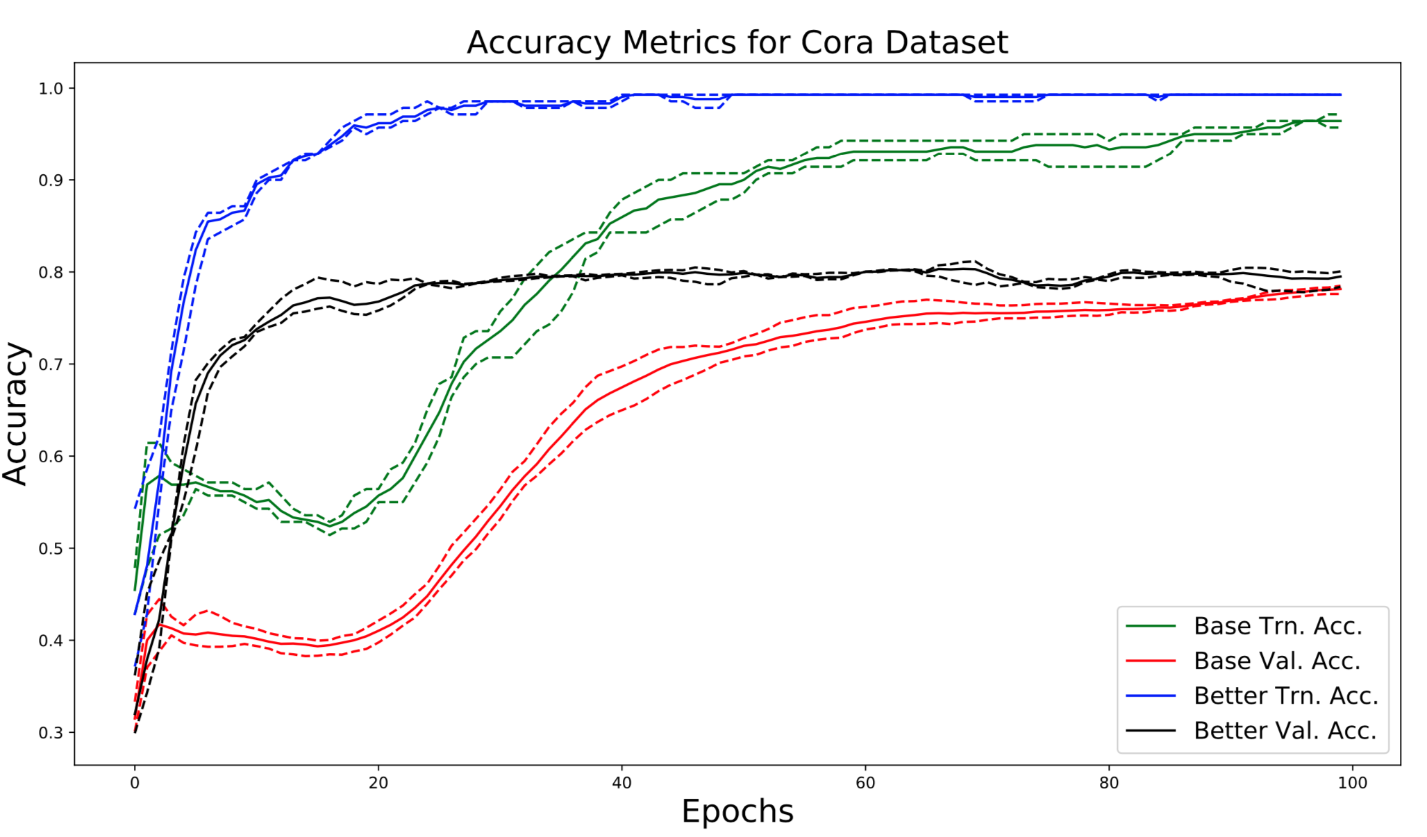
The performance of the improved model surpasses that of the baseline. All performance metrics associated with the improved model are superior to those of the baseline (Table 1). Even the training metrics of the proposed model improve, surpassing the baseline model with respect to both training loss and training accuracy. Finally, the proposed modifications to the model result in significantly improved accuracy on both training and validation sets (Figure 1, 2).

Convergence Time

The proposed modifications to the GAT model resulted in significantly faster convergence. The proposed model converged in around 20 epochs, while it took the baseline 100 epochs to converge (Figure 1). Similarly, on the Amazon Co-Purchase dataset, we observe that the proposed model modifications lead to convergence significantly earlier than the baseline. These gains in training efficiency supplement the gains in model performance, resulting in a model both more efficient and performant.

Training Stability

We improved training stability by adding layer normalization into intermediate layers of the GAT. We note that differences were especially noticeable on inductive tasks. Interestingly, the baseline model exhibits massive fluctuations in validation accuracy throughout training (Figure 3). Additionally, the model’s final performance varied greatly across trials (observed in the accuracy deviations in Figure 3). However, the proposed modifications to the model result in stable convergence to an optimum, yielding a solution that performs with comparatively little variation across trials.

Conclusion

In this post, we propose some modifications to the GAT architecture, inspired by best practices for transformers, which yield improved performance. These modifications; including layer normalization, attention normalization, projection of head output, and the addition of a separate classification layer; drastically improve the efficiency and performance of the GAT model in its original form. We show that these simple modifications increase performance, convergence time, and training stability of the model. We hope practitioners apply these practices to designing and implementing neural networks for graph-structured data.

Citations