 Blog Home
When are Neural Networks more powerful than Neural Tangent Kernels?
The empirical success of deep learning has posed significant challenges to machine learning theory: Why can we efficiently train neural networks with gradient descent despite its highly non-convex optimization landscape? Why do over-parametrized networks generalize well? The recently proposed Neural Tangent Kernel (NTK) theory offers a powerful framework for understanding these, but yet still comes with its limitations.
In this blog post, we are going to explore how we can analyze wide neural networks beyond the NTK theory, based on our recent Beyond Linearization paper and follow-up paper on understanding hierarchical learning. (This post is also cross-posted at off the convex path.)
Neural Tangent Kernels
The Neural Tangent Kernel (NTK) is a recently proposed theoretical framework for establishing provable convergence and generalization guarantees for wide (over-parametrized) neural networks (Jacot et al. 2018). Roughly speaking, the NTK theory shows that
- A sufficiently wide neural network trains like a linearized model governed by the derivative of the network with respect to its parameters.
- At the infinite-width limit, this linearized model becomes a kernel predictor with the Neural Tangent Kernel (the NTK).
Consequently, a wide neural network trained with small learning rate converges to 0 training loss and generalize as well as the infinite-width kernel predictor. A detailed introduction to the NTK can be found in this blog post on ultra-wide networks.
Does NTK fully explain the success of neural networks?
Although the NTK yields powerful theoretical results, it turns out that real-world deep learning do not operate in the NTK regime:
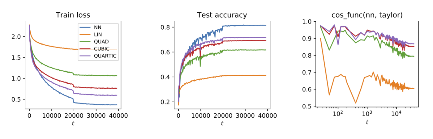
- Empirically, infinite-width NTK kernel predictors perform slightly worse (though competitive) than fully trained neural networks on benchmark tasks such as CIFAR-10 (Arora et al. 2019b). For finite width networks in practice, this gap is even more profound, as we see in Figure 1: The linearized network is a rather poor approximation of the fully trained network at practical optimization setups such as large initial learning rate (Bai et al. 2020).
- Theoretically, the NTK has poor sample complexity for learning certain simple functions. Though the NTK is a universal kernel that can interpolate any finite, non-degenerate training dataset (Du et al. 2018, 2019), the test error of this kernel predictor scales with the RKHS norm of the ground truth function. For certain non-smooth but simple functions such as a single ReLU, this norm can be exponentially large in the feature dimension (Yehudai & Shamir 2019). Consequently, NTK analyses yield poor sample complexity upper bounds for learning such functions, whereas empirically neural nets only require a mild sample size (Livni et al. 2014).
These gaps urge us to ask the following
Question: How can we theoretically study neural networks beyond the NTK regime? Can we prove that neural networks outperform the NTK on certain learning tasks?
The key technical question here is to mathematically understand neural networks operating outside of the NTK regime.
Higher-order Taylor expansion
Our main tool for going beyond the NTK is the Taylor expansion. Consider a two-layer neural network with $m$ neurons, where we only train the "bottom" nonlinear layer $W$:
$$
f_{W_0 + W}(x) = \frac{1}{\sqrt{m}} \sum_{r=1}^m a_r \sigma( (w_{0,r} + w_r)^\top x).
$$
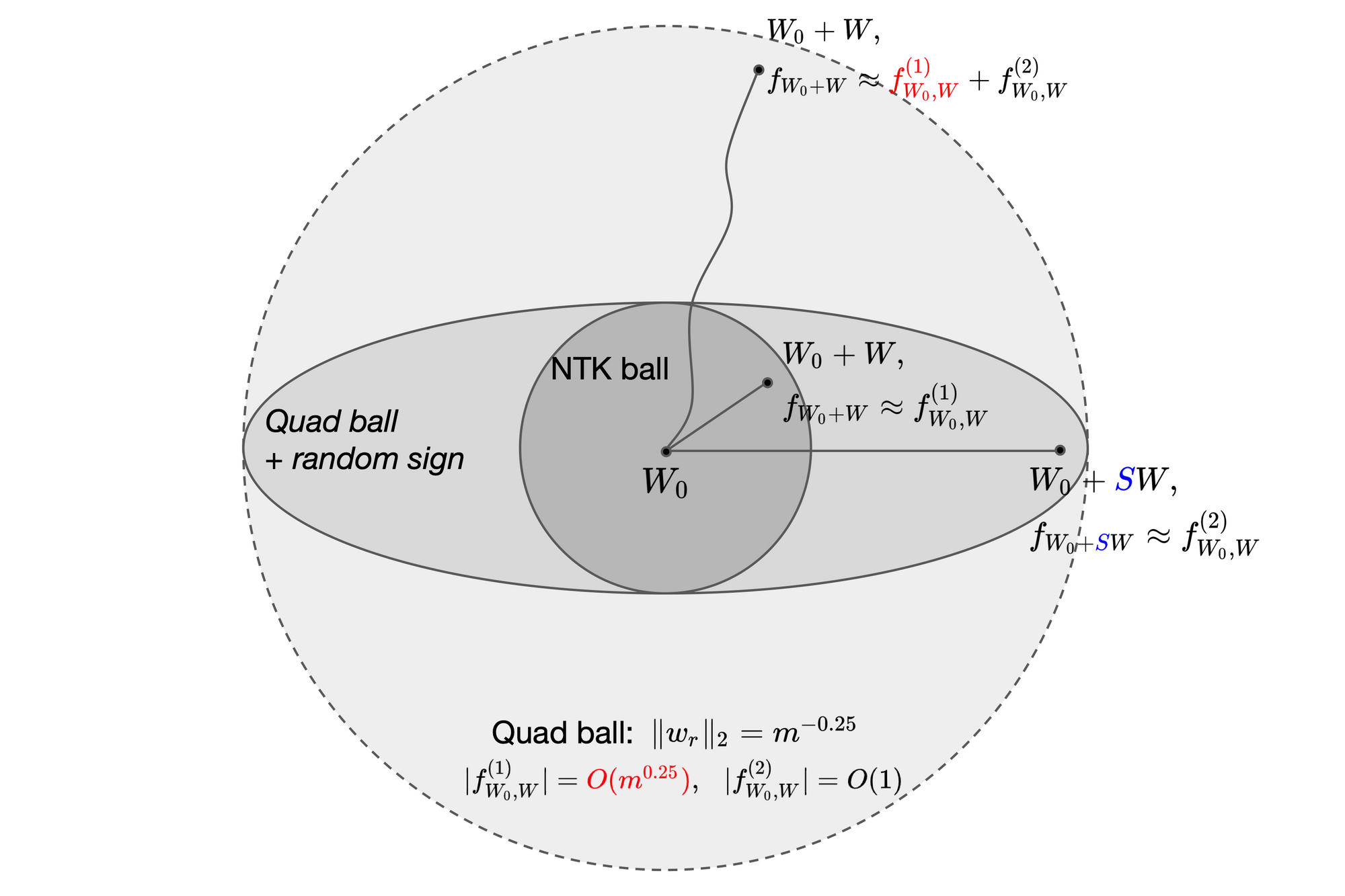
(Here, $W_0+W$ is an $m\times d$ weight matrix, where $W_0$ denotes the random initialization and $W$ denotes the trainable "movement" matrix initialized at zero). For small enough $W$, we can perform a Taylor expansion of the network around $W_0$ and get
$$
\begin{aligned}
f_{W_0+W}(x) & = \frac{1}{\sqrt{m}} \sum_{r=1}^m a_r \sigma(w_{0,r}^\top x) + \sum_{k=1}^\infty \frac{1}{\sqrt{m}} \sum_{r=1}^m a_r \frac{\sigma^{(k)} (w_{0,r}^\top x)}{k!} (w_r^\top x)^k \\
& := f^{(0)}_{W_0}(x) + \sum_{k=1}^\infty f^{(k)}_{W_0, W}(x).
\end{aligned}
$$
Above, $f^{(k)}_{W_0, W}(x)$ is the $k$-th order term in the Taylor expansion of $f$, and is a $k$-th order polynomial of the trainable parameter $W$. For the moment, let us assume that $ f^{(0)}_{W_0}(x)=0$ (this can be achieved via techniques such as the symmetric initialization).
The key insight of the NTK theory can be described as the following linearized approximation property
For small enough $W$, the neural network $f_{W_0,W}$ is closely approximated by the linear model $f^{(1)}$.
Towards moving beyond the linearized approximation, in our Beyond Linearization paper, we started by asking the following question:
Why just $f^{(1)}$? Can we also utilize the higher-order term in the Taylor series?
At first sight, this seems rather unlikely, as in Taylor expansions we always expect the linear term $f^{(1)}$ to dominate the whole expansion and have a larger magnitude than $f^{(2)}$ (and subsequent terms).
“Killing" the NTK term by randomized coupling
We bring forward the idea of randomization, which helps us escape the "domination" of $f^{(1)}$ and couple neural networks with their quadratic Taylor expansion term $f^{(2)}$. This idea appeared first in Allen-Zhu et al. (2018) for analyzing three-layer networks, and as we will show also applies to two-layer networks in a perhaps more intuitive fashion.
Let us now assign each weight movement $w_r$ with a random sign $s_r\in\{\pm 1\}$, and consider the randomized weights $\{s_rw_r\}$. The random signs satisfy the following basic properties:
$$
E[s_r]=0 \quad {\rm and} \quad s_r^2\equiv 1.
$$
Therefore, let $SW\in\mathbb{R}^{m\times d}$ denote the randomized weight matrix, we can compare the first and second order terms in the Taylor expansion at $SW$:
$$
E_{S} \left[f^{(1)}_{W_0, SW}(x)\right] = E{S} \left[ \frac{1}{\sqrt{m}}\sum_{r\le m} a_r \sigma'(w_{0,r}^\top x) (s_rw_r^\top x) \right] = 0,
$$
whereas
$$
f^{(2)}_{W_0, SW}(x) = \frac{1}{\sqrt{m}}\sum_{r\le m} a_r \frac{\sigma''(w_{0,r}^\top x)}{2} (s_rw_r^\top x)^2 = \frac{1}{\sqrt{m}}\sum_{r\le m} a_r \frac{\sigma''(w_{0,r}^\top x)}{2} (w_r^\top x)^2 = f^{(2)}_{W_0, W}(x).
$$
Observe that the sign randomization keeps the quadratic term $f^{(2)}$ unchanged, but "kills" the linear term $f^{(1)}$ in expectation!
If we train such a randomized network with freshly sampled signs $S$ at each iteration, the linear term $f^{(1)}$ will keep oscillating around zero and does not have any power in fitting the data, whereas the quadratic term is not affected at all and thus becomes the leading force for fitting the data. (The keen reader may notice that this randomization is similar to Dropout, with the key difference being that we randomize the weight movement matrix, whereas vanilla Dropout randomizes the weight matrix itself.)

Our first result shows that networks with sign randomization can still be efficiently optimized, despite its now non-convex optimization landscape:
Theorem: Any escaping-saddle algorithm (e.g. noisy SGD) on the regularized loss function $E_S[L(W_0+SW)]+R(W)$, with freshly sampled sign $S=S_t$ per iteration, can find the global minimum in polynomial time.
The proof of this result builds on the quadratic approximation $E_S[f]\approx f^{(2)}$, and recent understandings on neural networks with quadratic activation, e.g. Soltanolkotabi et al. (2017) & Du and Lee (2018).
Generalization and sample complexity: Case study on learning low-rank polynomials
We next study the generalization of these networks in the context of learning low-rank degree-$p$ polynomials:
$$
f_\star(x) = \sum_{s=1}^{r_\star} \alpha_s (\beta_s^\top x)^{p_s},~
|\alpha_s| \le 1,~\|(\beta_s^\top x)^{p_s}\|_{L_2} \le 1,~p_s\le p~\textrm{for all}~s.
$$
We are specifically interested in the case where $r_\star$ is small (e.g. $O(1)$), so that $y$ only depends on the projection of $x$ on a few directions. This for example captures teacher networks with polynomial activation of bounded degree and analytic activation (approximately), as well as constant depth teacher networks with polynomial activations.
For the NTK, the sample complexity of learning polynomials have been studied extensively in (Arora et al. 2019a), (Ghorbani et al. 2019), and many concurrent work. Combined, they showed that the sample complexity for learning degree-$p$ polynomials is $\Theta(d^p)$, with matching lower and upper bounds:
Theorem (NTK): Suppose $x$ is uniformly distributed on the sphere, then the NTK requires $O(d^p)$ samples in order to achieve a small test error for learning any degree-$p$ polynomial, and there is a matching lower bound of $\Omega(d^p)$ for any inner-product kernel method.
In our Beyond Linearization paper, we show that the quadratic Taylor model achieves an improved sample complexity of $\tilde{O}(d^{p-1})$ with isotropic inputs:
Theorem (Quadratic model): For mildly isotropic input distributions, the two-layer quadratic Taylor model (or two-layer NN with sign randomization) only requires $\tilde{O}({\rm poly}(r_\star, p)d^{p-1})$ samples in order to achieve a small test error for learning a low-rank degree-$p$ polynomial.
In our follow-up paper on understanding hierarchical learning, we further design a "hierarchical learner" using a specific three-layer network, and show the following
Theorem (Three-layer hierarchical model): Under mild input distribution assumptions, a three-layer network with a fixed representation layer of width $D=d^{p/2}$ and a trainable quadratic Taylor layer can achieve a small test error using only $\tilde{O}({\rm poly}(r_\star, p)d^{p/2})$ samples.
When $r_\star,p=O(1)$, the quadratic Taylor model can improve over the NTK by a multiplicative factor of $d$, and we can further get a substantially larger improvement of $d^{p/2}$ by using the three-layer hierarchical learner. Here we briefly discuss the proof intuitions, and refer the reader to our papers for more details.
Expressing polynomials: The way we approximate low-rank polynomials using quadratic Taylor models is similar as in the NTK analysis: we first express polynomials in the exact infinite-width kernel RKHS space, then convert the infinite-width representation to finite-width random feature representation using sampling + concentration bounds.
- Generalization bounds: We show that, while the NTK and quadratic Taylor model expresses functions using similar random feature constructions, their generalization depends differently on the norm of the input. In the NTK, the generalization depends on the L2 norm of the features (as well as the weights), whereas generalization of the quadratic Taylor model depends on the operator norm of the input matrix features $\frac{1}{n}\sum x_ix_i$ times the nuclear norm of $\sum w_rw_r^\top$. It turns out that this decomposition can match the one given by the NTK (it is never worse), and in addition be better by a factor of $O(\sqrt{d})$ if the input distribution is mildly isotropic so that $\|\frac{1}{n}\sum x_ix_i^\top\|_{\rm op} \le 1/\sqrt{d} \cdot \max \|x_i\|_2^2$, leading to the $O(d)$ improvement in the sample complexity.
- Hierarchical learning: The key intuition behind the hierarchical learner is that we can utilize the $O(d)$ sample complexity gain to its fullest, by applying quadratic Taylor model to not the input $x$, but a feature representation $h(x)\in \mathbb{R}^D$ where $D\gg d$. This yields a gain as long as $h$ is rich enough to express $f_\star$ and also isotropic enough to let the operator norm $\|\frac{1}{n}\sum h(x_i)h(x_i)^\top\|_{\rm op}$ be nice. In particular, for learning degree-$p$ polynomials, the best we can do is to choose $D=d^{p/2}$, leading to a sample complexity saving of $\tilde{O}(D)=\tilde{O}(d^{p/2})$.
Concluding thoughts
In this post, we explored higher-order Taylor expansions (in particular the quadratic expansion) as an approach to deep learning theory beyond the NTK regime. The Taylorization approach has several advantages:
- Non-convex but benign optimization landscape;
- Provable generalization benefits over NTKs;
- Ability of modeling hierarchical learning;
- Convenient API for expeirmentation (cf. the Neural Tangents package and the Taylorized training paper).
We believe these advantages make the Taylor expansion a powerful tool for deep learning theory, and our results are just a beginning. We also remark that there are other theoretical frameworks such as the Neural Tangent Hierarchy or the Mean-Field Theory that go beyond the NTK with their own advantages in various angles, but without computational efficiency guarantees. See the slides for more on going beyond NTK. Making progress on any of these directions (or coming up with new ones) would be an exciting direction for future work.
Resources
Our Papers:
Beyond Linearization: On Quadratic and Higher-Order Approximation of Wide Neural Networks (ICLR 2020).
Towards Understanding Hierarchical Learning: Benefits of Neural Representations (NeurIPS 2020).